Neural Style Transfer
Posted on Sun 19 March 2023 in data science, art
Neural Style Transfer
What is neural style transfer and how does it involve artificial intelligence?
Neural style transfer is a technique that takes a content image and style image and combines the two images so that the final output is in the style of the style image.
So, for example, I can take a content image. Then select a style image. To produce a third image with the imputed style.
| Content | Style | Generated |
|---|---|---|
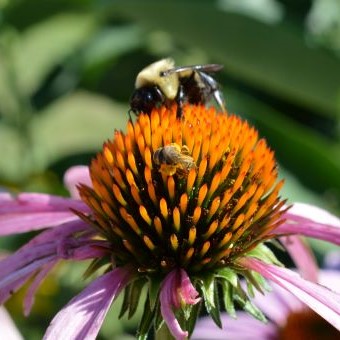 |
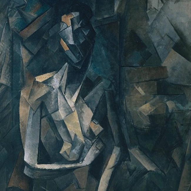 |
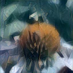 |
Alternatively, I can take the same photo and combine it with a style image that I created.
| Content | Style | Generated |
|---|---|---|
|
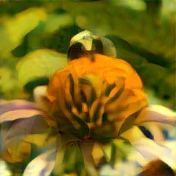 |
In this case, the style was one of my photographs that I manipuled using GIMP.
If you're interested in the art aspects, please check out my art blog at www.heatheranndye.com.
The Picasso image is Figure dans un Fauteuil and in the US is no longer considered to be under copyright.
Demonstration App
This technique utlizes a convolutional neural network (CNN) such as VGG-19 which has the capability to recognize 1000 object classes. We utilitze the ability of the CNN to recognize patterns in order to perform style transfer.
From an artist's perspective, this technique can utilize AI in a manner that does not result in copy right theft.
You can construct your own neural style transfer using the streamlit app. The original source code for this project is at https://github.com/heatheranndye/ImageToStyle.
References and motivation
The original motivation for this project was to explore Fast Api and the diffusers at Hugging Face during my participation in the the PyBites Developer Mindset Program.
I used these references to construct the application.
How is Neural Style Transfer Performed?
We successively apply the layers of the CNN to the content and style images; then harvest the output layers immediately prior to the max pooling. (These output layers are matrices.) In the case of the VGG19 model, there are five such layers. The idea in the CNN is that each successive layer captures more complicated characteristics of the image.
The generated image is initially set equal to the content image and then is modified to take on characteristics of the style image.
Let \(C^k _{ij}\) denote the \(k\)-th output layer of the content image, \(G^k _{ij}\) denote the \(k\)-th output of the generated image, and \(A^k_{ij}\) denotes the \(k\)-th output of the style file. In the selected model, there are five possible layers to harvest occuring before max pooling.
For the content layers, we let \(O_c\) denote the output layers selected to optimize the content. For the style layers, we let \(O_s\) denote the output layers selected from the selected from the style image. We need to select at least one layer of each type, keeping in mind that the later layers capture more sophisticated characteristics.
We denote the content loss function as \(\mathit{L}_c $. Then
We sum these two functions to obtain the total loss:
Here is a code snippet.
 style_loss = 0
    for value in style_layers:
        counter = value - 1
        # print(f"{counter}")
        batch, channel, height, width = gen_feat[counter].shape
        genitem = gen_feat[counter]
        styleitem = style_feat[counter]
        G = torch.mm(
            genitem.view(
                channel,
                height * width,
            ),
            genitem.view(channel, height * width).t(),
        )
        A = torch.mm(
            styleitem.view(
                channel,
                height * width,
            ),
            styleitem.view(channel, height * width).t(),
        )
        style_loss += F.mse_loss(G, A)
    return style_loss
Notice the choice of \(A^T A\) in the style loss function. This ensures that the loss function has some flexibility as explained below.
Why are the loss functions different?
I don't know how the authors of the paper selected the different loss functions. But I can reflect on the why the choice was made. Let's consider the simplest version of our problem. We have a picture consisting of a single pixel. Let's assume grayscale for simplicity. Our content image is represented by \((0)\) and our style image is represented by \((1)\). Our goal is to generate a third image that minimizes the distance between \((0)\) and \((1)\). Remember that our generated image is initially the content image, so we'll represent the content image as \(h\).
Then our loss function is \(L = (h)^2 + (1-h)^2\). Rewriting this loss function, we find that \(L = 2h^2 + 1 - 2h\), meaning that for this simplistic case the minimum is at the halfway point (\(1/2\)) between the two values.
Now let's consider a function that utilizes a transpose in conjunction with the style image.
The product of a single entry matrix and its transpose is a square, so
\(L = h^2 + (1^2-h^2)^2\) and we see that the minimum is \(\frac{1}{\sqrt{2}}\). So this result is a bit closer to the content image than the style image.
In practice, we'll be working with large matrices and the interesting part is matrix multiplication is not unique - that is if \(A^T A = B\), there may be more than one solution for \(A\). The matrix multiplication will mean that the actual loss function for style will be more complicated and have more flexibility.
Training the Model
Once the output layers are selected, you can train the model using the code below.
 for e in range(100):
        gen_features = model(generated_image)

        total_loss = calculate_loss(
            content_features,
            gen_features,
            style_features,
            style_layers=style_layers,
            content_layers=content_layers,
        )
        # optimize the pixel values of the generated
        # image and backpropagate the loss
        optimizer.zero_grad()
        total_loss.backward()
        optimizer.step()
        # print the image and save it after each 100 epoch
        # if e / 100:
        # print(f"e: {e}, loss:{total_loss}")
Which output layers?
You'll notice that the code snippet above specifies the output layers used in the content and style loss. What layers were selected? In the images that I generated, I selected the layers recommended in the original paper. For content, I selected layer 5. For the style layers, I selected all five layers. However, you can use the streamlit app to experiment with the layers and determine which works best. If you'd like to experiment with your own photos, you can download the code at https://github.com/heatheranndye/ImageToStyle/blob/master/ImageToStyle/photo_mod/styletransfer.py.