Hello Data!
Posted on Wed 26 October 2022 in data science
Hello data science!
In this article, we'll create a small simulation and explore confidence intervals and the central limit theorem.
We frequently talk about 95% or 90% confidence intervals but what information do these intervals give us?
The Central Limit Theorem
Given a population with mean \(\mu\) and standard deviation \(\sigma\), the distribution of sample means \(\left( \frac{\sum x}{n} = \bar{x} \right)\) with sample size \(n\) will be approximately normally distributed for sufficiently large \(n\).
Given a few semesters of calculus and linear algebra, it can be shown that:
-
\(E(\bar{x}) = \mu\)
-
\(Var(\bar{x})=\frac{\sigma^2}{n}\)
Then, we hit another roadblock: proving that for sufficiently large \(n\), the sampling distribution is approximately normal. Even after going through the proof, it can be really difficult to think about what this means in practice. So, we'll construct some examples using Python.
We'll start by importing the packages used in this demonstration.
import random
import pandas as pd
import matplotlib.pyplot as plt
from scipy.stats import t
from numpy import sqrt
Generate some data and build a confidence interval, Round 1
We'll start by generating some fake data from a continuous, uniform distribution on the interval \([0,10]\) with a sample size of 50. The mean, \(\mu\), of this distribution is 5 and the standard deviation is approximately 2.9. The sufficiently large part of the Central Limit Theorem means that the sample size must be 30 or larger if the underlying distribution is not normal. I'll set the random seed so that this data is reproducible.
random.seed(42)
mydata = pd.Series([random.uniform(0,10) for i in range(50)])
For right now, let's pretend that we don't know the specifics of the distribution that we sampled. (Because in reality, you wouldn't.) First, inspect the five number summary using the describe method. Notice that the median (\(\tilde{x}\)) is 4.63 and the sample mean is 4.5. Based on the quartiles, this data set is symmetric.
Next, we examine the sample standard deviation which is 2.9. This means that if the data comes from a normal distribution then about 68% of my data should fall in the interval \((1.6, 7.4)\). Using the describe function, I only have access to \(P_{25}\) and \(P_{50}\), so I'll investigate a little further.
mydata.describe()
count    50.000000
mean      4.506842
std       2.932888
min       0.064988
25%       2.190886
50%       4.636386
75%       6.927794
max       9.731158
dtype: float64
We can check the quantiles of the data set to see that \(P_{16} \approx 0.96\) and \(P_{84} \approx 8.06\) This suggests that our data is not normal, but we can also visually confirm this by examining a histogram of the data.
mydata.quantile(q=0.16), mydata.quantile(q=0.84)
(0.9608109148093343, 8.060286952634595)
mydata.hist()
<AxesSubplot: >
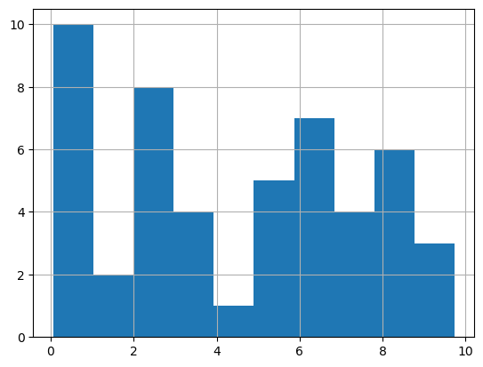
This visual inspection confirms that our data is not normal, but luckily! we are working with a sample of size 50.
The formula for the confidence interval of a sample mean is:
The \(t_{\alpha /2, df}\) refers to a the critical value, a value on the x-axis of the Student-t distribution that cuts off a tail of area \(\alpha /2\) and the \(df\) refers to the degrees of freedom which specifies a specific t-distribution. (Fun fact: The Student-t distribution was derived by William Seally Gossett who, at the time, was employed by the Guinness Brewery.)
Python can quickly compute this formula. We use SciPy's t.ppf to obtain the critical value. We compute a 90% confidence interval, which means that
and
xbar = mydata.mean()
mysd = mydata.std()
(xbar - mysd/ sqrt(len(mydata)) * t.ppf(0.95, len(mydata)-1), xbar + mysd/ sqrt(len(mydata)) * t.ppf(0.95, len(mydata)-1))
(3.8114545041480343, 5.202230430974262)
Confidence Intervals, Round 2
Now, we can investigate what exactly the confidence level means beyond selecting the critical value. The first thing that we'll do is write a small function to automatically compute our confidence interval.
def student_t_confidence(data, conf_level):
    xbar = data.mean()
    mysd = data.std()/sqrt(len(data))
    alpha_2 = (1-conf_level)/2
    tsig = t.ppf(0.95, len(data)-1)
    return (xbar - mysd*tsig, xbar+mysd*tsig )
Here is our brand new function in action.
student_t_confidence(mydata, 0.90)
(3.8114545041480343, 5.202230430974262)
Next, we're going to generate 20 samples of size 50 and store them in a data frame.
Here is a function that accomplishes this goal.
def make_some_fake_data(sample_count: int, sample_size: int):
    local_df = pd.DataFrame()
    for i in range(sample_count):
        local_list =[random.uniform(0,10) for j in range(sample_size)]
        local_df[f"sample {i}"]=local_list
    return local_df


mydf = make_some_fake_data(20, 50)
Here is the head of my new data frame.
mydf.head()
| sample 0 | sample 1 | sample 2 | sample 3 | sample 4 | sample 5 | sample 6 | sample 7 | sample 8 | sample 9 | sample 10 | sample 11 | sample 12 | sample 13 | sample 14 | sample 15 | sample 16 | sample 17 | sample 18 | sample 19 | |
|---|---|---|---|---|---|---|---|---|---|---|---|---|---|---|---|---|---|---|---|---|
| 0 | 3.701810 | 0.114810 | 9.951494 | 9.689963 | 3.161772 | 9.039286 | 9.811497 | 4.421598 | 8.972081 | 6.222570 | 6.906144 | 0.856130 | 1.843637 | 6.476347 | 3.232738 | 2.828390 | 8.723830 | 9.926920 | 7.242167 | 0.993546 |
| 1 | 2.095070 | 7.207218 | 6.498781 | 9.263670 | 7.518645 | 5.455903 | 5.362157 | 2.137014 | 7.436554 | 0.269665 | 6.272424 | 7.200747 | 0.513767 | 9.084114 | 9.701847 | 2.985558 | 0.358991 | 2.952308 | 9.799422 | 6.856803 |
| 2 | 2.669778 | 6.817104 | 4.381001 | 8.486957 | 0.725431 | 8.345950 | 9.392371 | 4.731862 | 4.746744 | 3.940203 | 1.019013 | 4.885778 | 9.410636 | 8.266312 | 4.041751 | 5.869377 | 0.684207 | 9.779445 | 9.672697 | 5.444659 |
| 3 | 9.366546 | 5.369703 | 5.175758 | 1.663111 | 4.582855 | 5.825096 | 1.153418 | 9.011808 | 2.591915 | 5.643920 | 7.724809 | 7.581647 | 4.777292 | 0.714098 | 5.145963 | 9.989023 | 6.311610 | 6.582298 | 8.045876 | 9.778425 |
| 4 | 6.480354 | 2.668252 | 1.210042 | 4.856411 | 9.984544 | 1.480938 | 9.704006 | 7.960248 | 2.472397 | 0.271020 | 8.502932 | 6.906093 | 8.221156 | 1.659228 | 9.881192 | 4.896403 | 9.209291 | 2.744804 | 3.657750 | 3.586738 |
Here, we take our 20 samples and compute a confidence interval for each sample. The results are stored in a dictionary, using the sample number as the key.
ci_dict = {}
for j in range(mydf.shape[1]):
    results = student_t_confidence(mydf.iloc[:,j], 0.9)
    ci_dict.update({j:results})
We analyze the results of our computations and count the number of intervals that actually contain the true population mean, 5. Our goal in computing these intervals is to estimate the true population mean.
def count_the_good_ones(local_dict, truemean):
    count = 0
    for i in range(len(local_dict)):
        therange = local_dict.get(i)
        if therange[0] < truemean and therange[1]> truemean:
            count +=1
    return count

thenum = count_the_good_ones(ci_dict, 5)
print(thenum)
17
And, only 17 intervals actually contain the true population mean.
So what just happened? Let's take a look at a visualization.
plt.plot([5 for i in range(20)], color= 'k')
themins = [ci_dict.get(i)[0] for i in range(20)]
plt.plot(themins, 'bs')
themaxes = [ci_dict.get(i)[1] for i in range(20)]
plt.plot(themaxes, 'rs')
themeans = [(themins[i] + themaxes[i])/2 for i in range(20)]
plt.plot(themeans, 'D')
for i in range(20):
    plt.vlines(x=i, ymin=themins[i], ymax=themaxes[i])
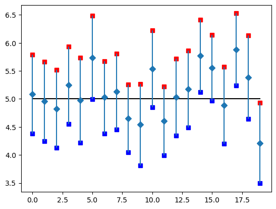
The three intervals that do not contain the true population mean have sample means that are relatively far from the true sample mean. The sample means were in the tails of the sampling distribution, meaning that in those cases, we were unlucky and obtained a sample that did not represent the actual population that the sample was drawn from.
This occurrs even if we collect all our data correctly.
With a 90% confidence interval, if you repeatedly collected samples of the same size and constructed confidence intervals, only 90% of the intervals contain the true population mean.
In my simulation, we know the true population mean is five, so we can correctly pick out the bad confidence intervals.
In reality, we have no way of knowing if our confidence interval is a good confidence interval or a bad confidence interval.